Evaluation of results
Final output data is obtained in the evaluation branch, during which the model under consideration (or rather, its characterisation through base solutions obtained from the calculation) is evaluated under specific thermal boundary conditions.
While thermal coupling coefficients, heat source distribution and weighting factors are boundary condition independent, further output data is dependant on air temperatures of spaces calculated and, in the event that heat source elements have been included in the model, power density values, which all must be assigned as a boundary conditions to these respective base solution cases as well.
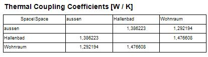
Thermal coupling coefficients matrix and heat source distribution factors
 As
the direct result of the computation the matrix of
thermal coupling
coefficients is provided. For a two dimensional model the matrix shows
length related transmittance L2D [Wm−1K−1]
; for three dimensional construction the matrix displays thermal coupling
coefficients L3D per se [WK−1]. Because thermal
coupling coefficients - and as such elements of the conductance matrix -
are independent from particular boundary conditions,
the matrix itself can be output prior to any user input of temperatures.
As
the direct result of the computation the matrix of
thermal coupling
coefficients is provided. For a two dimensional model the matrix shows
length related transmittance L2D [Wm−1K−1]
; for three dimensional construction the matrix displays thermal coupling
coefficients L3D per se [WK−1]. Because thermal
coupling coefficients - and as such elements of the conductance matrix -
are independent from particular boundary conditions,
the matrix itself can be output prior to any user input of temperatures.
Based on the output of thermal coupling coefficients one can calculate the thermal transmittance values (linear thermal transmittance Ψ (Psi) for two dimensional linear thermal bridges (see Psi-Value Determination), or point thermal transmittance χ (chi) for the three dimensional point thermal bridges).
In the event heat sources are available also, the distribution factor of each source is shown too - like the thermal coupling coefficients this values are independent from boundary conditions also. If N spaces are attached to the considered construction the distribution table will shown N numbers. The i-th (i = 1,N) value of the distribution table shows the percentage of the heat provided by the particular heat source passing to the i-th space. The values of the distribution table are therefore from the range 0 to 1; because the steady state calculation does not cover the heat capacity storage, the sum of all distribution values must result in 1 (apart from minor rounding errors).
Dynamic, transient problems, in which the heat storage capacity is taken into account, result in the output of harmonic, periodic coupling coefficients, also calculated directly and not dependant from any particular boundary conditions, are output as a matrix for each specific period length chosen. This results can be used for the analysis of dynamic behaviour of the component for example to read out amplitudes and phase shifts / time lags (like Lpe needed within Passivhaus Projektierungspaket PHPP) or to calculate effective mass capacities.
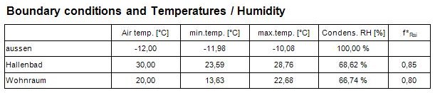
Boundary conditions
Any further evaluation requires the definition of boundary conditions - these are specified by air temperatures of spaces connected to the building component and all power densities of all heat sources. Only after that data has been provided further results can be requested.
Temperature extremes, dew points, fRsi-temperature factors, g-values
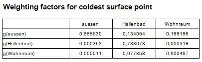
As soon as the boundary conditions have been applied, the application determines locations on the surfaces of all spaces of the model at which the minimum temperature is reached for given boundary conditions. The report "Results" lists coordinates of such points together with the value of the temperature at that point, the dew point value [1] resulting from that temperature and the corresponding temperature factor fRsi. The temperature weighting factors ("g–values") are also output for these coldest points. It is worth to mention, that the temperature weighting factors are independent from the boundary conditions. Contrary, the location of coldest surface points is dependant on the boundary conditions chosen, and therefore the output of weighting factors for coldest points can be provided after boundary conditions have been set.
According to the standard conformance requirement of EN ISO 10211 the "Results report" can b output to the printer.
For some special purpose it might be desirable to receive some output of the
distribution of g-values within the building construction or at it surfaces.
This is possible within the evaluation stage also. By using the nature of g-values,
which in particular are base solution values, the user has to assign the
boundary condition of the base solution of interest to 1 to receive the kind of
"temperature distribution" showing the g-values themselves. The output can then
show isolines, false coloured images or visualizations of "surface g-values" for
example.
Finally, the output of f-values is also possible because those are
special case of g-values.
See also: Evaluations and Results